Forecasting the Next Trading Day in SPX (Hourly)

Why probabilities beat point forecasts

Single-price forecasts can be misleading. A model can be directionally correct while missing magnitude, or land close to the close while being wrong about risk. Instead of asking for the exact next candle, I asked a more useful question: where is SPX likely to end up after the next seven hourly candles, and with what probability?

What I built

The model outputs a probability distribution over the next-day move. That lets me compute trading-style probabilities like:

P(Δ7 ≥ +10 points)
P(Δ7 ≤ -10 points)
P(|Δ7| ≤ 10 points)

This framing matches how traders think: ranges, probabilities, and risk bands rather than a single deterministic close.

Dataset

I used hourly SPX OHLC candles. Each row is one hour of open, high, low, and close. The model looks back 120 hours (about 3-4 weeks of trading hours) and predicts the move over the next 7 hourly candles, which is one full trading day. Training data spans May 15, 2019 at 10:30 AM ET through January 23, 2026 at 3:30 PM ET.

Turning forecasting into classification

Instead of predicting a future close, I predict the future point move after seven hours and discretize it into bins.

Future move

Δ₇ = Close_t+7 - Close_t

BIN_SIZE = 5 | MAX_MOVE = 200

Bins cover [-200, +200] → 80 total bins

Each label is a single bin index. The CNN then outputs an 80-bin softmax distribution for the next-day move.

Windowing setup

WINDOW = 120, HORIZON = 7. Each input is a 120-hour feature matrix.

Shapes

X ∈ R^{120 x F}

y ∈ {0, 1, ..., 79}

Each sample uses 120 hours of history to classify the 7-hour move bin.

Model architecture: fast ResNet-style Conv1D

A small ResNet-style CNN gave the best balance of accuracy, speed, and stability. It is parameter-efficient and trains quickly on hourly candles.

Stem: Conv1D(32, k=5) + BN + LeakyReLU + SpatialDropout
Residual blocks: 2x ResBlock(32) → MaxPool → 2x ResBlock(64) → MaxPool → ResBlock(128)
Head: GlobalAvgPool → Dense(64) → Dense(80, softmax)

The fast ResNet-style Conv1D produces a probability distribution over 80 bins for the next-day move.

Training details

Time split: first 80% train, last 20% test.
StandardScaler fit on training only.
Batch size 1024, epochs 20 with early stopping.
Loss: sparse categorical cross entropy.
Optimizer: Adam (lr = 1e-3).
Callbacks: EarlyStopping(patience=4), ReduceLROnPlateau(patience=2).

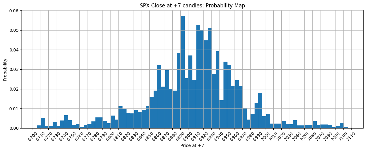
Probability map outputs

The output is a full histogram of likely Δ7 outcomes. From that histogram I compute bullish, bearish, and chop-day probabilities. The histogram below reflects the latest available data as of January 23, 2026 at 3:30 PM ET.

SPX close at +7 candles probability map histogram — Histogram output lets you compute directional or range probabilities.

CNN vs Transformer results

I tested a Transformer model on the same task. It consistently lagged the CNN on short-horizon errors.

CNN errors

Step +1 RMSE: 23.0

Step +5 RMSE: 51.0

Transformer errors

Step +1 RMSE: 24.0

Step +5 RMSE: 53.2

Why CNNs won on this dataset

CNNs assume local, reusable patterns, which matches candle behavior.
Transformers need more data to learn locality from scratch.
CNNs trained faster, so iteration and tuning were more productive.

Automating the pipeline (next step)

Append new hourly candles to the dataset.
Fine-tune the model on CPU for a few epochs.
Generate the next-day probability map.
Publish the histogram and JSON to the site.

Final takeaways

Predict distributions, not point estimates.
Small CNNs can outperform larger models on realistic datasets.
Probability outputs align better with trading decisions.

Sources

arXiv: 2512.21804

This post is educational only. Trading decisions should be made with professional advice and your own risk controls.

Forecasting the Next Trading Day in SPX (Hourly) with a Probability CNN